Classification: Neural

Lab setup

First, make sure you have completed the initial setup.

Open Terminal. Run the update command to make sure you have the latest code.
```
$ mwc update
```

Move to this lab's directory.

$ cd ~/Desktop/making_with_code/mwc2/unit3/lab_classification_neural

Move to your MWC directory.
```
$ cd ~/Desktop/making_with_code
```

Get a copy of this lab's materials.

git clone https://git.makingwithcode.org/mwc/lab_classification_neural.git

This lab picks up immediately from the classification_features lab. Students bring what they learned there—feature engineering, logistic regression, evaluation metrics—and discover that those tools are insufficient for image classification. That failure motivates neural networks.

How this lab meets the learning objectives

Classification techniques (Classification with features through Convolutional Neural Networks): Rather than survey a grab-bag of unrelated algorithms, this lab walks a single spectrum from fully hand-designed to fully learned: logistic regression on hand-picked features, logistic regression on raw pixels, a multi-layer perceptron, and a convolutional neural network. Each step changes exactly one thing—who designs the features, and how much the model learns on its own—so students can attribute performance differences to a specific, nameable cause rather than to "a different algorithm." The side-by-side comparison (same data, same evaluation, four points on that spectrum) is what makes "how does the computer decide?" concrete.

Hyperparameter tuning (throughout): Hidden layer sizes and training epochs in the MLP, training epochs in the CNN, and the architectural choices—kernel size, number of filters, pooling—sketched and discussed in Convolutional Neural Networks are all hyperparameters (or close cousins of them) with a measurable effect on performance. Students tune at least one and document the results.

ANNs (Artificial Neural Networks): Students examine the architecture of a single perceptron and an MLP before running one. The perceptron sketch and MLP diagram activities ensure students understand the structure before treating it as a black box.

CNNs (Convolutional Neural Networks): Students trace an image through convolutional and pooling layers before training a CNN. The comparison with MLP (same data, different architecture) makes the design choice concrete and measurable.

Sample digits from the MNIST dataset

In the previous lab you built a spam classifier in three stages: you wrote rules by hand, then handed the model a handful of features you designed, and finally let it choose from every word in the vocabulary and learn which ones mattered. Each stage traded human cleverness for trust in the learning algorithm—and each one did better than the last.

Now we face a harder problem: classifying handwritten digits. MNIST is the classic benchmark dataset of handwritten digits. It contains 70,000 grayscale images, each 28×28 pixels. Each pixel's brightness is stored as a number between 0 (black) and 1 (white), so the input for each example is a 2-dimensional array (28×28) of these brightness values—784 numbers in all.

Classification with features

💻 Load and visualize some examples:

$ digits --explore

This prints a few digits as ASCII art and shows the label distribution. (Add a number to see more examples, for example digits --explore 10)

In the spam lab, you designed features like "contains_free" and "number of exclamation marks." You knew what patterns to look for because you had read lots of spam messages.

What features might you design for handwritten digits? Some examples might include:

Total number of bright pixels
The fraction of bright pixels in the top half vs. the bottom half
Pixel brightness in different parts of the image
Whether the digit has a closed loop

Implement some of your features in models/features.py (look for the extract_features method) and evaluate the result:

$ digits models.features.FeatureClassifier -a

👾 💬 numpy

Pixel values are provided as a numpy array, which is like a list but much more powerful.

13    def extract_features(self, pixels):
14        img = pixels.reshape(28, 28)
15        return {
16            "mean_brightness": float(pixels.mean()),
17            "top_half_brightness": float(img[:14, :].mean()),
18        }

We won't go into all the details right now, but a few tips for writing your features:

Line 14 calls reshape, which reshapes the list of values (pixels) into a 2-dimensional square (img).
Line 17 has an example of how to select part of the 2-dimensional array: you have to provide two slices, the first specifying which rows you want and the second specifying which columns you want. 7:14 means 7 through 14 (not including 14), :4 means everything up to 4, : means "all."
Numpy arrays have lots of useful methods. Both of the provided features use mean, which takes the average of all the contents. Other useful methods include max, min, and sum.

Every pixel a feature

Let's borrow an intuition from the previous lab--instead of guessing which words mattered, you made every word a feature and let logistic regression to sort out which ones were useful. Here, you could just hand all 784 raw pixel values straight to LogisticRegression and let it learn a weight for each one.

👁 Open models/pixels.py. There's no FeatureExtractor, no DictVectorizer, no Pipeline—just a LogisticRegression that takes the pixel arrays directly:

 4class PixelClassifier:
 5    def fit(self, X, y):
 6        self._classifier = LogisticRegression(max_iter=1000)
 7        self._classifier.fit(X, y)
 8        return self
 9
10    def predict(self, X):
11        return self._classifier.predict(X)

💻 Run it:

$ digits models.pixels.PixelClassifier

Artificial Neural Networks

Learned features

Think back to a feature you might design for digit classification—say, the average brightness in the left quarter of the image. You could write it as a function that takes in all 784 pixel values and returns a single number:

    def extract_features(self, pixels):
        img = pixels.reshape(28, 28)
        return {
            "left_brightness": float(img[:, :7].mean())
        }

Look at what that function actually does: it multiplies each pixel by either 1 (if it's in the left quarter) or 0 (if it isn't), adds up the results, and scales them down. That's a weighted sum—the same calculation that has driven every classifier you've built so far—except here you chose the weights, by hand, before training even began: 1 for the pixels you decided mattered, 0 for the rest.

But weights don't have to be chosen by hand. You already know how to learn them—logistic regression does it through training, starting from nothing and gradually adjusting. So: what if, instead of deciding in advance which of the 784 pixels should count toward a feature, the model started with random weights for all of them and adjusted those weights through training—the very same way it already learns to weigh the features at the end of the pipeline?

Now imagine doing that many times over: building a whole bank of these candidate-feature functions, each starting from its own random weights, each free to become whatever weighted combination of pixels turns out to help. Train the entire system together, and the model isn't just learning how to weigh a set of features you handed it—it's learning what those features should be in the first place.

That's the idea behind a multi-layer perceptron (MLP): place a layer of these learned-feature functions in front of the final decision-making layer. It's the same move this lab keeps making, taken one level deeper—replacing a step you used to do by hand with something the model works out for itself.

Structure of a single neuron

Each of those candidate-feature functions is called a neuron (originally inspired by the structure of neurons in your brain). A neuron takes several inputs, multiplies each by a (learnable) weight, adds them up along with a bias term, and passes the result through an activation function:

$$ \text{output} = \text{activation}(x_1 w_1 + x_2 w_2 + \cdots + x_n w_n + b) $$

If "sum + bias" looks familiar, it should—that's the calculation that drove every classifier in the spam lab and the pixel classifier above. The only new ingredient is the activation function, which processes the neuron's output. (We won't go into the details here.)

A neuron, in other words, is a learned feature: a measurement the network invented for itself, the same way left_third_brightness was a measurement you invented for yourself. The difference is that you can name and explain your feature, while a learned one is just whatever pile of weights happened to reduce the loss.

A single hidden layer

The simplest possible MLP places one layer of neurons—a hidden layer—between the input and the output:

MLP with a single hidden layer

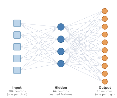
Each of the 64 hidden neurons computes its own weighted sum of all 784 pixel values, applies its activation function, and passes the result forward. Then each neuron in the output layer combines those 64 learned features into a probability that the image is a particular digit.

💻 Train an MLP with 32 neurons:

$ digits models.mlp.MLPClassifier --hidden 32

You should see accuracy climb with each epoch:

Training MLP (hidden_sizes=(32,), epochs=10)
  epoch  1/10  loss=1.125  val_accuracy=0.854  2.1s
  epoch  2/10  loss=0.441  val_accuracy=0.895  2.0s
  ...
  epoch 10/10  loss=0.168  val_accuracy=0.924  2.0s

💻 Try a few other hidden layer sizes and training lengths:

$ digits models.mlp.MLPClassifier --hidden 16
$ digits models.mlp.MLPClassifier --hidden 256
$ digits models.mlp.MLPClassifier --hidden 64 --epochs 20

Multi-layer perceptrons

Nothing requires stopping at one hidden layer. A multi-layer perceptron stacks several of them, so that one layer's output becomes the next layer's input:

MLP with two hidden layers

Pause on this diagram before moving on. A few questions worth working through together:

Where are the weights? Every line in the diagram is a weight—a number the model adjusts during training. Each hidden neuron in layer 1 has one weight per input pixel (784 weights), plus a bias. With 128 neurons that's already around 100,000 numbers in just the first layer. Ask students to estimate the total number of weights across all layers; the sheer scale tends to land.

How is the forward pass calculated? Each neuron computes the same thing: multiply each incoming value by its weight, add them all up, add a bias, and pass the result through an activation function. The output of one layer becomes the input to the next—so the forward pass is just repeating that calculation layer by layer until you reach the output.

Weights as matrices. This lab intentionally avoids matrix notation to keep the focus on ideas rather than notation. Students who know matrices may recognize that all the weights going into a layer can be organized as a matrix, and the forward pass through that layer is a single matrix multiplication. If that observation comes up, it's worth affirming: this is exactly how PyTorch (and every other deep learning library) stores and computes with weights—matrices are the implementation that makes neural networks fast.

Simple math, enormous scale. Every individual calculation in a neural network is elementary—multiply two numbers, add them to a running total. What makes neural networks computationally demanding isn't the complexity of any single operation; it's the sheer number of them. This is precisely why GPUs are so effective for training and running neural networks: a GPU is designed to execute millions of simple arithmetic operations in parallel, which is exactly the workload a forward or backward pass produces.

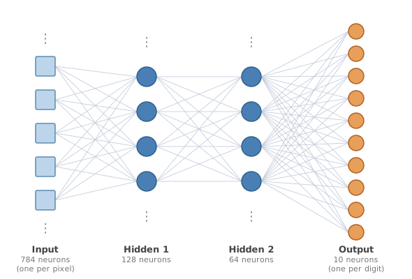
Each additional layer gets to learn features of the previous layer's features—combinations of combinations. A first hidden layer might settle on something like edges and curves; a second can combine those into more complex shapes; and so on, until the output layer has rich enough material to make a confident decision.

Backpropagation

How does an MLP learn its weights—now spread across several layers instead of just one? The training algorithm is called backpropagation, and—like logistic regression—it is built from an idea you already understand: start with a bad model, measure how bad it is, and nudge it to be a little less bad, over and over.

Start by choosing random numbers for every weight, in every layer.
Measure how bad the model is. Take each image in the training set, pass it through the network layer by layer, and compare the prediction it produces to the true label. As in logistic regression, each wrong (or under-confident) prediction earns a penalty, and all the penalties get added up into a single loss—just now averaged over ten possible digits instead of two message classes.
Use calculus to figure out which direction to nudge each weight to bring that loss down. Here is the wrinkle a layered network adds: a weight in the first layer affects the final answer only indirectly—its effect passes through every layer that comes after it. So the algorithm works backward through the network: first it figures out how wrong the output layer's guesses were, then uses that to work out how much blame each neuron in the hidden layer just before it deserves, then steps back again to the layer before that, assigning blame and computing nudges all the way back to the first layer. That backward pass through the layers is what gives the algorithm its name: backpropagation.
Repeat steps 2 and 3 for thousands of examples.

💻 Train a deeper MLP, with two hidden layers:

$ digits models.mlp.MLPClassifier --hidden 128 64

Training MLP (hidden_sizes=(128, 64), epochs=10)
  epoch  1/10  loss=0.852  val_accuracy=0.890  2.3s
  epoch  2/10  loss=0.321  val_accuracy=0.905  2.2s
  epoch  3/10  loss=0.246  val_accuracy=0.917  2.2s
  ...
  epoch 10/10  loss=0.054  val_accuracy=0.947  2.2s

💻 Compare it to your best single-hidden-layer result, and try a few more architectures. Hidden layers can be any size you want, but multiples of 2 are most efficient.

$ digits models.mlp.MLPClassifier --hidden 256 128 64
$ digits models.mlp.MLPClassifier --hidden 64 64 --epochs 20

ANNs. Backpropagation isn't the point here; what matters is that students understand the structure (inputs, weights, bias, activation function, output; single perceptron; MLP layers) and the function (the network learns from data). The walkthrough above gives both without requiring calculus, in the same numbered-steps style used for logistic regression in the previous lab—worth pointing out explicitly, so students see that this "scary" algorithm is built from a familiar pattern.

It's worth having students sketch a single perceptron and a multi-layer perceptron by hand. Rather than another on-computer step, this is a good candidate for a five-minute, off-the-keyboard activity: have groups sketch both on paper or a whiteboard before training one—labeling inputs, weights, the activation function, and (for the MLP) the layers and their sizes. Sketching by hand tends to surface exactly the gaps in understanding that running working code glosses over.

Hyperparameter tuning. Architecture is itself a hyperparameter here: depth (number of layers) and width (neurons per layer) interact in ways that size alone, in the single-hidden-layer checkpoint, didn't show. Two networks with a similar total neuron count can perform quite differently depending on how those neurons are arranged into layers—worth surfacing if a group is comparing, say, --hidden 128 64 against --hidden 64 64 64.

Convolutional Neural Networks

Detecting local patterns

The MLP can learn its own features—but it learns them by looking at the whole 784-pixel image at once. It would be better if the model could learn features about parts of the image: small, local patterns like straight lines, loops, corners, and curves.

If you looked at just a small patch of an image, you could probably hand-write a detector for patterns like these—"is there a horizontal edge in this corner of the patch?" is the kind of question you could answer by comparing a handful of neighboring pixel values. But you already know how that story ends: hand-written features lose to learned ones.

So: what if the model learned these small-patch pattern-detectors itself—and then went looking for each one everywhere in the image, not just in one fixed spot? That's the idea behind a convolutional neural network (CNN).

Kernels

A convolutional layer applies a small function (called a kernel) across the image. The kernel slides over every position and multiplies the current pixels by the kernel's weights, transforming the pixel values into an activation map that shows where that pattern appears.

For example, a horizontal-edge-detecting kernel might produce high values wherever there is a horizontal line in the image, and low values elsewhere. The network doesn't know in advance which patterns will be useful—the kernel values themselves are learned, by backpropagation, the same way features in hidden layers of the ANN were learned.

The kernel size controls how large a patch the kernel examines at each position. A 3×3 kernel looks at a 3×3 patch of pixels; a 5×5 kernel sees more context but uses more parameters and is slower to compute. Smaller kernels (3×3) are most common in modern CNNs.

Stride controls how far the kernel moves at each step. Stride 1 means it moves one pixel at a time. With stride 2, it skips every other position—so a kernel applied to a 28×28 image with stride 2 produces a roughly 13×13 activation map instead of a 26×26 one. Each additional convolutional layer with stride 2 halves the spatial dimensions again.

You may already recognize this idea: it's the same as the step argument in range. range(0, 28, 1) visits every position; range(0, 28, 2) skips every other one.

CNNs. Students should come away knowing the basic architecture (input, convolutional layers, activation functions, pooling layers, fully connected layers, output) and the effect of number of layers, kernel size, stride, activation function, and loss function.

The starter code here uses stride to reduce spatial dimensions rather than separate pooling layers—it's one fewer concept to introduce, and students already know stride from range. You may wish to mention max pooling briefly as an alternative approach that has similar spatial-reduction effects, and note that both are common in real architectures.

As with the perceptron and MLP earlier, the architecture is best addressed with paper and pencil rather than another on-screen step: have students sketch the CNN architecture diagrammed above, labeling the input layer (size), each convolutional layer (number of filters, kernel size, and stride), the fully connected layer, and the output layer. Comparing sketches in small groups is a quick way to surface confusions about what each layer's numbers mean before moving on.

Students do not need to know how the kernel values are learned (backpropagation through a convolution is beyond scope—and, if the on-ramp above landed, they already have the right intuition: it's the same backward-blame-assignment process, just threading through a different kind of layer). What matters is that the kernel values are learned, the effect of kernel size on what the network can see, and how stride controls the output size.

Train a CNN

💻 Train the CNN:

$ digits models.cnn.CNNClassifier

Training CNN (epochs=5)
  epoch  1/5  loss=0.628  val_accuracy=0.938  8.3s
  epoch  2/5  loss=0.145  val_accuracy=0.969  8.1s
  ...
  epoch  5/5  loss=0.048  val_accuracy=0.971  8.0s

Training takes longer than the MLP (a few minutes on a laptop). You can reduce epochs to get results faster, at some cost to accuracy:

$ digits models.cnn.CNNClassifier --epochs 3

By default, digits trains on 10,000 examples to keep iteration fast. Add --full to train on all 60,000 examples in MNIST—accuracy goes up, but training takes roughly six times as long:

$ digits models.cnn.CNNClassifier --full

Try it on your own handwriting

Once you have a CNN you're happy with, it's worth saving it—training takes several minutes, and you don't want to repeat that every time you want to use the model.

💻 Save your trained model's configuration and weights:

$ digits models.cnn.CNNClassifier --save cnn

Next time, you can load the saved model by name instead of re-training:

$ digits cnn

💻 Now point your trained classifier at the real world. Find a piece of paper, write a digit on it in thick marker, and hold it up to your computer's camera:

$ digits cnn --run

A window opens showing your camera's view with a green box drawn on it. Whatever falls inside that box is converted into a 28×28 image—the same format as the MNIST images you trained on—and classified on the spot. The terminal prints the predicted digit and the model's confidence, updating live as you move the paper around. Press q (with the camera window focused) to quit.

Discussion prompts

On model selection:

Hand-picked features, raw pixels, MLP, and CNN all solve the same problem—which one you should use depends on context. What factors would lead you to choose each?
Modern image classifiers use CNNs with dozens of layers (ResNet, VGG). What challenges might arise when training a very deep network?
Architectural ideas like convolution mattered, but a lot of the dramatic progress in machine learning over the last decade came from something more mundane: bigger networks, trained on much larger datasets. If scale is such a big part of what makes a model good, who can afford to build the best ones—and what does that suggest about how the field will keep developing?

On interpretability:

Logistic regression on hand-picked features is fairly interpretable—you can point to a specific feature and its weight and say "this is why." CNNs are not. When does interpretability matter more than raw accuracy? (Medical diagnosis? College admissions? Hiring?)
What would it mean for a digit classifier to be unfair? Are some digits harder to classify than others? Are some handwriting styles less well represented in the training data?